@katiejolly6
on
On struggling with aes(): an intro to writing functions with ggplot outputs
Last week I was trying to programmatically create plots and came across so many errors! Mostly I was not understanding why my variables weren’t translating from inputs in my function to inputs for ggplot2. After I figured out my error it seemed simple, but I’m hoping my issues figuring it out can be useful to other people, so you don’t have to spend as much time on it!
tl;dr
aes_string is super useful for including plots in user defined functions and can take your plots to a whole new level!
Introducing my problem
For this example, to make it more reproducible, I’ll use data from Fivethirtyeight’s early senate poll data in their Github repository.
library(tidyverse) # general tasks
library(broom) # tidy model output
library(ggthemes) # style the plots

poll_data <- read_csv("https://raw.githubusercontent.com/fivethirtyeight/data/master/early-senate-polls/early-senate-polls.csv")

glimpse(poll_data)
## Observations: 107
## Variables: 4
## $ year                  <int> 2006, 2006, 2006, 2006, 2006, 2006, 2006...
## $ election_result       <int> -39, -10, -9, -16, 40, 10, -2, -41, -31,...
## $ presidential_approval <int> 46, 33, 32, 33, 53, 44, 37, 39, 42, 33, ...
## $ poll_average          <int> -28, -10, -1, -15, 39, 14, 2, -22, -27, ...
The corresponding article Early senate polls have a lot to tell us about November. essentially found that there is a strong correlation between polling numbers and the ultimate result of an election, and a slight smaller correlation between presidential approval and election results.
This post will focus more on the behind-the-scenes plotting than on the modeling, because there are plenty of awesome models already out there!
Essentially, I was making lots of plots with lots of models and wanted a better way to automate plots for evaluating model assumptions. Instead of copy/pasting each time, it would be so much easier to write my own function. So that’s what I did! Ultimately it probably would have been faster to just type everything out, but now I know how to better use ggplot2 in future problems.
A function and a model
For this example I’ll use a linear model that models election_result by poll_average.
poll_lm <- lm(election_result ~ poll_average, data = poll_data)

summary(poll_lm)
##
## Call:
## lm(formula = election_result ~ poll_average, data = poll_data)
##
## Residuals:
##      Min       1Q   Median       3Q      Max
## -29.4281  -5.0197   0.5601   6.1364  17.9357
##
## Coefficients:
##              Estimate Std. Error t value Pr(>|t|)
## (Intercept)  -0.89110    0.76969  -1.158     0.25
## poll_average  1.04460    0.03777  27.659   <2e-16 ***
## ---
## Signif. codes:  0 '***' 0.001 '**' 0.01 '*' 0.05 '.' 0.1 ' ' 1
##
## Residual standard error: 7.93 on 105 degrees of freedom
## Multiple R-squared:  0.8793, Adjusted R-squared:  0.8782
## F-statistic:   765 on 1 and 105 DF,  p-value: < 2.2e-16
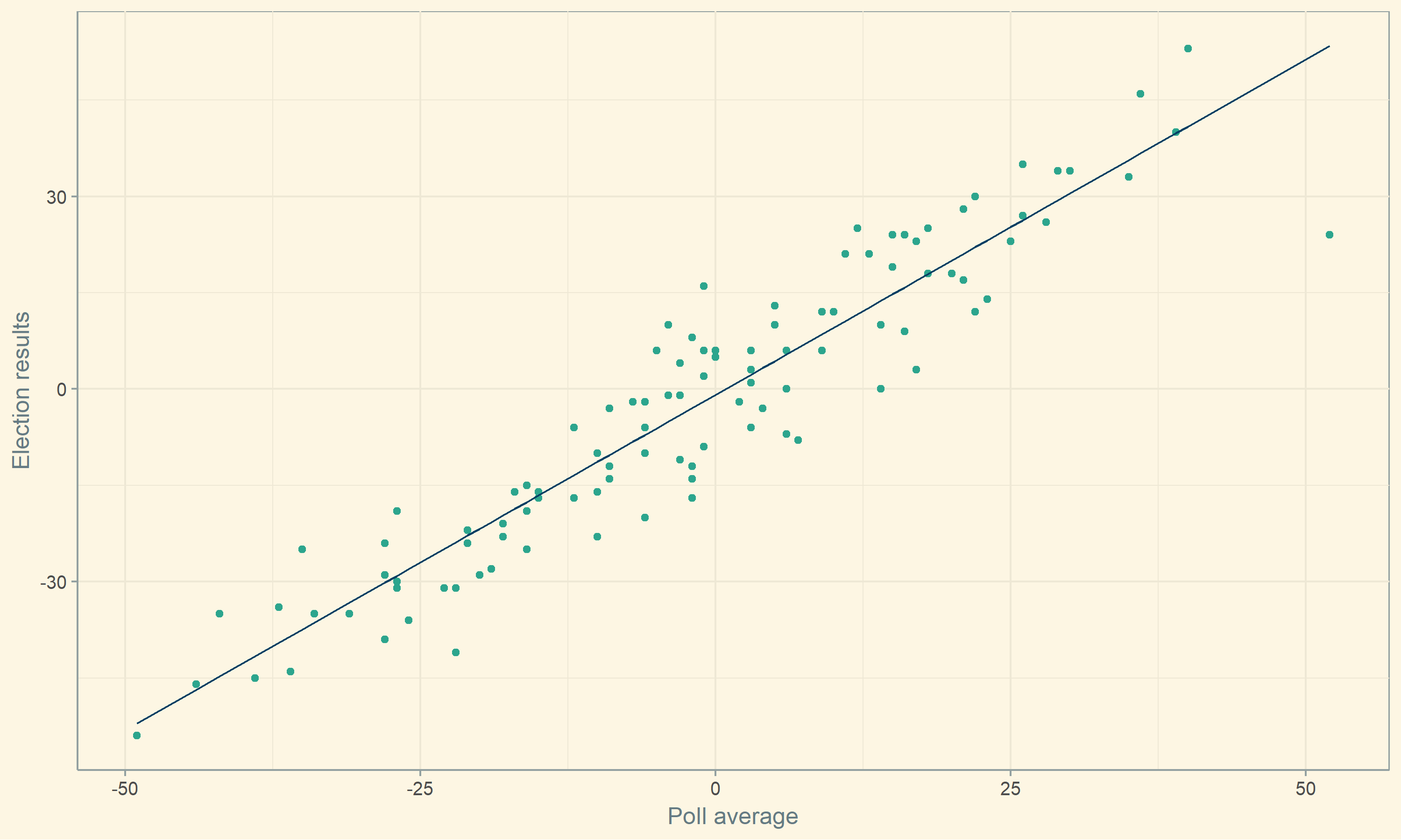
I’m just going to focus on plotting the resulting line with the original data points.
I knew the code I needed to create the plot.
augment(poll_lm) %>%
  ggplot() +
    geom_point(aes(x = poll_average, y = election_result), color = "#2CA58D") +
    geom_line(aes(x = poll_average, y = .fitted), color = "#033F63") +
    theme_solarized() +
    theme(axis.title = element_text()) +
    labs(x = "Poll average", y = "Election results")

But I wanted a way to have a function that takes the model, response, and explanatory variables!
At first I wrote this:
plot_model <- function(mod, explanatory, response) {
  augment(mod) %>%
  ggplot() +
    geom_point(aes(x = explanatory, y = response)) +
    geom_line(aes(x = explanatory, y = .fitted)) +
    theme_solarized() +
    theme(axis.title = element_text()) +
    labs(x = "Poll average", y = "Election results")
}
When I tried to run it, I got an error that was a bit confusing at first.
plot_model(poll_lm, poll_average, election_result)
## Error in FUN(X[[i]], ...): object 'poll_average' not found
Basically it couldn’t find the poll_average variable. I checked the spelling so many times, I thought I was going crazy.
After googling around, I struck gold with the ggplot2 article Define aesthetic mappings programatically It suggested a few aes variations and I decided to go with aes_string() to be able to use string inputs in my function.
So, I tried again.
plot_model <- function(mod, explanatory, response, .fitted = ".fitted") {
  augment(mod) %>%
  ggplot() +
    geom_point(aes_string(x = explanatory, y = response), color = "#2CA58D") +
    geom_line(aes_string(x = explanatory, y = .fitted), color = "#033F63") +
    theme_solarized() +
    theme(axis.title = element_text()) +
    labs(x = "Poll average", y = "Election results")
}

plot_model(poll_lm, "poll_average", "election_result")
Ta-da! Even though this is a simple example, it will be so helpful for me in the future! I’m sure there are other ways to solve this problem, so I’d love to know your favorite fix for programming with ggplot2.
Edit:
Per comments, I’ve edited the function to be more applicable to other models!
plot_model <- function(mod, explanatory, response, .fitted = ".fitted") {
  augment(mod) %>%
  ggplot() +
    geom_point(aes_string(x = explanatory, y = response), color = "#2CA58D") +
    geom_line(aes_string(x = explanatory, y = .fitted), color = "#033F63") +
    theme_solarized() +
    theme(axis.title = element_text()) +
}

plot_model(poll_lm, "poll_average", "election_result") + labs(x = "Poll average", y = "Election results")
Running this code would give the same plot, just without the hardcoded axis labels.