@katiejolly6
on
Mapping DC's urban farms and gardens
I made spring rolls for dinner with vegetables I got from the market (some of them, at least) and it reminded me of how much I love urban agriculture. It also reminded me of how much I love spring rolls on a nice spring day. I volunteered for a while at an urban farm last summer and it still amazes me that we were able to grow so much fresh food in such a small space. As someone who has always lived in an [sub]urban place, I feel very removed from my food when I go to the grocery store.
A few weeks ago I was talking to a friend about how much urban farming and gardening there was in Washington, DC. Apart from DC, the other half of my life is spent in Saint Paul, MN where there is also quite a bit of urban agriculture. We decided to look online to see what sorts of numbers we could find about urban farming in DC and I thought it would be worthwhile to map! I was interested to see what parts of the city have the largest farm areas. My expectation is that Shaw/Howard and SW Waterfront areas both have a lot of farms because those are the neighborhoods I hear about most.
Libraries and Data Gathering
# load libraries

library(sf)
library(geojsonio)
library(tidyverse)
library(extrafont)
Most of the data for this project comes from DC’s open data site. I used the API endpoints for the geoJSON format because I find those relatively easy to work with in R using {geojsonio}.
I’m sure there’s an easier way to read in a geoJSON in as an sf object, but the way I know how to do it involves converting it from an sp object. To make this a bit faster (and to comply with D.R.Y.) I’ll write a simple function for it. Since all of the data is in DC, I’ll transform it to the UTM zone 18N now so that the projections don’t get confused later.
geojson_read_sf <- function(url) {
  geojson_read(url, what = "sp") %>% # read in as sp
    st_as_sf() %>% # convert to sf
    st_transform(32618) # UTM zone 18n
}
First I’ll read in the urban farm locations. Per the documentation, this data includes
urban agriculture sites in the District of Columbia. These are distinguished from community gardens in that they are generally not intended for the public to use the space for their own growing activities, and in that many have a commercial focus.
Essentially, these are functioning farms as opposed to hobby gardens.
urban_farms_sf <- geojson_read_sf("https://opendata.arcgis.com/datasets/4a28f83e5d624bd6986b2b534a5d4dc9_55.geojson")
I also want to include data on community gardens. From the documentation these include
active community gardens in the District of Columbia. These generally fall into three operating categories: DC Department of Parks and Recreation (DPR), National Parks Service (NPS), and independent.
community_gardens_sf <- geojson_read_sf("https://opendata.arcgis.com/datasets/a82537b01c2141558ba5e9e13224d395_4.geojson")
For this particular project I chose not to include the school gardens.
For the last piece of data, I want a background map of DC. I’ll create this with a few different basemaps.
# dc wards from http://opendata.dc.gov/datasets/ward-from-2012

dc_wards_sf <- geojson_read_sf("https://opendata.arcgis.com/datasets/0ef47379cbae44e88267c01eaec2ff6e_31.geojson")

# major roads from http://opendata.dc.gov/datasets/major-roads/geoservice

dc_roads_sf <- geojson_read_sf("https://opendata.arcgis.com/datasets/3031b2c72a4942bb86356e921e73e8c3_38.geojson")

# national parks from http://opendata.dc.gov/datasets/national-parks

dc_nat_parks_sf <- geojson_read_sf("https://opendata.arcgis.com/datasets/14eb1c6b576940c7b876ebafb227febe_10.geojson")

# dc boundary line from http://opendata.dc.gov/datasets/washington-dc-boundary

dc_boundary_sf <- geojson_read_sf("https://opendata.arcgis.com/datasets/7241f6d500b44288ad983f0942b39663_10.geojson")

# water from {tigris}

dc_water_sf <- tigris::area_water(state = "District of Columbia", county = "District of Columbia", year = 2015) %>%
  st_as_sf() %>%
  st_transform(32618)
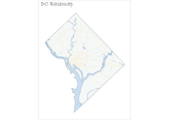
DC Basemap
In order to create all of the maps, I wanted to have one standardized basemap of DC. I like using the geom_sf() function from {ggplot2} for geographic data plotting, so we’ll use that method for this map. For interactive maps I like using {leaflet}.
To make the plot easier, I also set a general theme that I can re-use. If you don’t want to use {extrafont}, the fonts will be the default font instead of the specified one, and the rest of the plot will still work!
map_theme <-
  theme(
    panel.grid.major = element_line(colour = "transparent"),
    axis.line = element_blank(),
    axis.text = element_blank(),
    axis.ticks = element_blank(),
    axis.title = element_blank(),
    panel.background = element_blank(),
    panel.border = element_blank(),
    panel.grid = element_blank(),
    panel.spacing = unit(0, "lines"),
    legend.justification = c(0, 0),
    title  = element_text(family = "Bradley Hand ITC", size = 15),
    legend.title = element_text(family = "Century Gothic", size = 9),
    legend.text = element_text(family = "Century Gothic", size = 8),
    legend.background = element_blank(),
    legend.position="none", # legend is not really necessary
    plot.caption = element_text(family = "Century Gothic", size = 8, hjust = 0, color = "gray60"),
    plot.subtitle = element_text(family = "Century Gothic", size = 8, vjust = -2, color = "gray60"),
    plot.background = element_rect(color = "#d4dddc")
  )

farm_green <- "#869727"
street_yellow <- "#F5EDC1"
non_profit_pink <- "#FE6C69"
for_profit_teal <- "#64ACAB"
To create the basemap, I overlayed the boundary, water features, and main roads with the custom theme.
dc_basemap <- ggplot() +
  geom_sf(data = dc_wards_sf, fill = "#d4dddc", color = NA, alpha = 0.2) +
  geom_sf(data = dc_roads_sf, color = street_yellow, alpha = 0.5) +
  geom_sf(data = dc_boundary_sf, fill = NA, color = "#909695") +
  geom_sf(data = dc_water_sf, fill = "#cbdeef", color = "#9bbddd") +
  map_theme + # the theme I created
  labs(title = "DC Basemap")

dc_basemap
Urban farms
First, I want to know where all of the urban farms in DC are located. Again, this includes farms that are (often) for-profit and business-oriented.
First, I’ll try zooming to the extent of the farm layer. From prior knowledge I know that it’s nearly impossible to see the farms at the full extent of the city because they’re so small.
I use range() and st_coordinates() because I saw it in Ryan Peek’s Mapping with sf: part 2 blog post and it seemed to work well for my purposes, too.
mapRange_farms <- c(range(st_coordinates(urban_farms_sf)[,1]),range(st_coordinates(urban_farms_sf)[,2])) # find the max and min for x and y coordinates, creates a vector. c(x min, x max, y min, y max)

dc_basemap +
  geom_sf(data = urban_farms_sf, fill = farm_green) +
  coord_sf(xlim = mapRange_farms[c(1:2)], ylim = mapRange_farms[c(3:4)]) +
  labs(title = "DC's Urban Farms",
       subtitle = "Extent zoomed to farm layer") +
  theme(plot.subtitle = element_text(vjust = 1))
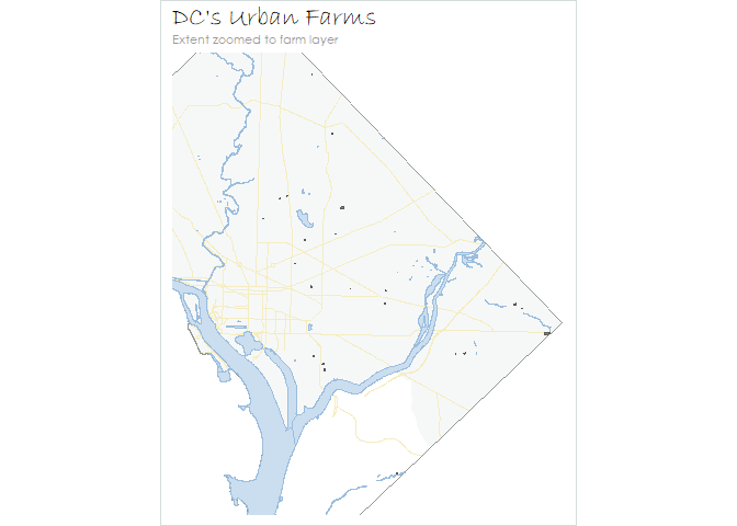
It’s still pretty hard to see the farms in this map, they’re much too small (because they’re life-size, so to speak).
Instead, I’ll use proportional symbols at the centroid of each farm using st_centroid(). A really helpful feature of this function is that it just replaces the geometry column with the centroid (so it keeps all of the other variables!). Either that’s a new feature, or I don’t remember that from using the function in the past.
urban_farms_point_sf <- st_centroid(urban_farms_sf) # add point geometry

dc_basemap +
  geom_sf(data = urban_farms_point_sf, aes(size = 2 * ACREAGE), color = farm_green, alpha = 0.7) +
  labs(title = "DC's Urban Farms",
       subtitle = "Size proportional to acreage",
       caption = "By Katie Jolly // 28 May 2018 \nData from opendata.dc.gov")
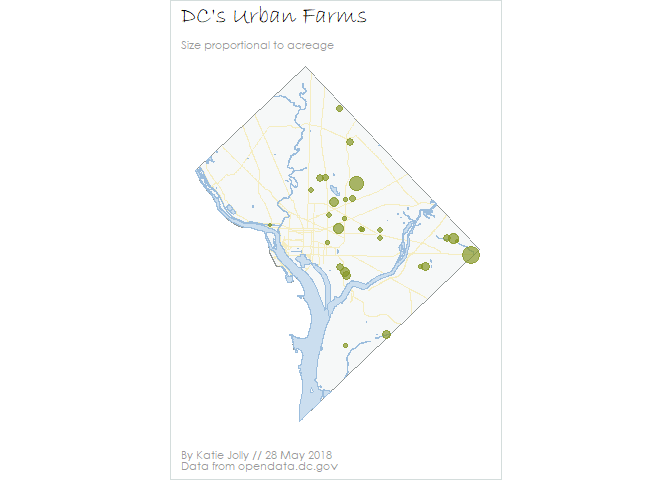
So it looks like there are larger farms near Shaw/Howard and the eastern corner of the city. There are also quite a few near the downtown area!
Now I’m curious as to where the for-profit and not-for-profit farms are in the city.
dc_basemap +
  geom_sf(data = urban_farms_point_sf, aes(size = 2 * ACREAGE, color = STATUS), alpha = 0.7) +
  scale_color_manual(breaks = c("For-profit", "Non-profit"), values = c(for_profit_teal, non_profit_pink)) +
  labs(title = "DC's Urban Farms",
       subtitle = "Size proportional to acreage",
       caption = "By Katie Jolly // 28 May 2018 \nData from opendata.dc.gov") +
  annotate("text", x = 319000, y = 4305000, label = "Non Profit Farm", size = 2, family = "Century Gothic", color = non_profit_pink) +
  annotate("text", x = 318900, y = 4304000, label = "For Profit Farm", size = 2, family = "Century Gothic", color = for_profit_teal)
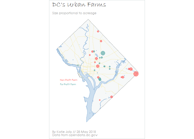
I was surprised at how (seemingly) clustered the types of farms are! I’m now wondering if there is a grant program or other incentive in certain neighborhoods that make non-profit farms more likely to start there.
Another explanation could be that there are some for profit farms with multiple locations (like Cultivate the City). Perhaps those farms are all in certain areas of the city.
cultivate_the_city <- urban_farms_point_sf %>%
  filter(COMPANY == "Cultivate the City")

dc_basemap +
  geom_sf(data = cultivate_the_city, aes(size = 2 * ACREAGE), color = for_profit_teal, alpha = 0.7) +
  labs(title = "Cultivate the City Farms",
       subtitle = "Size proportional to acreage",
       caption = "By Katie Jolly // 28 May 2018 \nData from opendata.dc.gov")
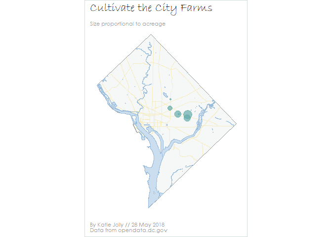
Based on this look at one farm, it seems like the last hypothesis (that multiple locations of for profit farms tend to cluster) might be a good start. I’d have to look at more farms to be sure, but I’m satisfied with this answer for now.
Community Gardens
I’m also interested in seeing where the community gardens are in DC. I’ll use a similar map to show those!
The size of the symbol will be proportional both to make it comparable to the farm map and because not every garden has the number of plots listed for various reasons.
community_gardens_point_sf <- st_centroid(community_gardens_sf) # add point geometry

dc_basemap +
  geom_sf(data = community_gardens_point_sf, aes(size = 2 * ACRES), color = farm_green, alpha = 0.7) +
  labs(title = "DC's Community Gardens",
       subtitle = "Size proportional to acreage",
       caption = "By Katie Jolly // 28 May 2018 \nData from opendata.dc.gov")
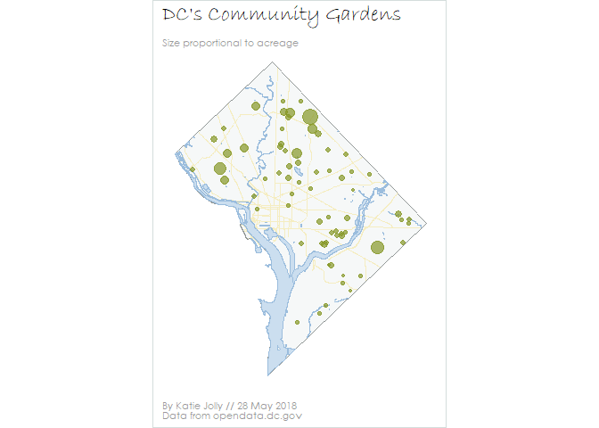
While the urban farms were more concentrated in the NE and SE quadrants of DC, it looks like community gardens are more spread out. Some of the largest ones are in NW (near-ish to Tenleytown), near Takoma/Manor Park, and east of the Anacoostia River in a Fort Circle Park.
Concluding thoughts
In the future I’d love to expand the maps to include features like green roofs, instead of just urban farms and gardens. In reality, sustainability and food encompass a lot more than just what I’ve already mapped. I’d also like to include some other variables like park land and zoning codes to explain why some of the patterns in placement exist. As for my guess that SW Waterfront would have more farms, I now expect that it would have more alternatives like green roofs.
Creating these maps also helped me practice more of the {sf} functions and making/designing maps with {ggplot2}. I’ve been working through Geocomputation with R so it was great to put some of that to use! One of my goals for this upcoming year is to learn more about the design aspects of data visualization, so I spent far more time than I usually would have on color and font selection :)
Have some good resources for designing nice plots in R? Send them my way!